8 A Post-Kaleckian Distribution and Growth Model

Overview

The post-Kaleckian growth model was developed by Bhaduri and Marglin (1990) and others to synthesise Marxian and Keynesian ideas about the effects of income distribution on economic growth.¹ According to the Marxian view, capital accumulation is driven by profits. By contrast, Michal Kalecki and post-Keynesians such as Nicholas Kaldor argued that a redistribution of income towards profit-earners is likely to reduce consumption, as workers tend to have a higher marginal propensity to consume than capital owners. The post-Kaleckian growth model integrates these two mechanisms in a Keynesian framework in which aggregate demand and growth are demand-determined. It allows for wage-led as well as profit-led demand and growth regimes. In a wage-led regime, a redistribution of income towards workers has expansionary effects on aggregate demand (and possibly growth) as the expansionary effect on consumption outweighs the negative effect on investment. In a profit-led regime, the effect is contradictory as investment falls by more than consumption rises. Whether a regime is wage- or profit-led depends on the relative size of the propensities to consume and the propensity to invest.

This is a model of long-run steady state growth. In the steady state, all endogenous variables grow at the same rate.² Changes in parameters or exogenous variables lead to an instantaneous adjustment of the model’s variables, so that the model can be analysed like a static one. We consider a version of the model with linear functions based on Hein (2014), chap. 7.2.2.

The Model

\[ r=h \frac{u}{v} \tag{8.1}\]

\[ s=[s_W + (s_\Pi - s_W)h]\frac{u}{v}, \quad 0 \geq s_W > s_\Pi \geq 1 \tag{8.2}\]

\[ c= \frac{u}{v}-s \tag{8.3}\]

\[ g=g_0+g_1u+g_2h, \quad g_i > 0 \tag{8.4}\]

\[ u=v(c+g) \tag{8.5}\]

where \(r\), \(s\), \(c\), \(g\), and \(u\) are the profit rate, the saving rate, the consumption rate, the investment rate, and the rate of capacity utilisation, respectively.

Equation 8.1 decomposes the profit rate into the product of the profit share \(h\) (total profits over total output), the rate of capacity utilisation (actual output over potential output), and the inverse of \(v\) (the capital-potential output ratio). Let \(Y\) be output, \(K\) be the capital stock, and \(Y^P\) be potential output, the decomposition can also be written as \(r=\frac{\Pi}{K}=\frac{\Pi}{Y}\frac{Y}{Y^P}\frac{Y^P}{K}\). The profit share and the capital-potential output ratio are taken to be exogenous in this model. Note also that the wage share is given by \(1-h\). By Equation 8.2, the economy-wide saving rate is given by the sum of saving out of wages (\(s_W(1-h)\frac{u}{v}\)) and saving out of profits (\(s_\Pi h\frac{u}{v}\)). It is assumed that workers have a higher marginal propensity to consume than capital owners (\(s_W>s_\Pi\)). Equation 8.3 simply states that consumption is income not saved. According to Equation 8.3, investment is determined by an autonomous component \(g_0\) that may capture Keynesian `animal spirits’, by the rate of capacity utilisation, and by the profit share. While the rate of capacity utilisation is a signal of (future) demand, the profit share may stimulate investment as internal funds are typically the cheapest source of finance. Finally, Equation 8.5 is an equilibrium condition that assumes that the rate of capacity utilisation adjusts to clear the goods market.

The key question addressed by this model is a how a change in the profit share affects the rate of capacity utilisation and the rate of growth.³ As shown formally in the analytical discussion below, there is no unambiguous answer to this question as the model encompasses different regimes. Three main regimes can be identified. First, a regime in which both the rate of utilisation and the rate of growth are negatively affected by an increase in the profit share. We will call this a wage-led demand and growth regime (WLD/WLG). Second, a regime in which the rate of utilisation is negatively affected and the rate of growth is positively affected by an increase in the profit share. We will call this a wage-led demand regime and profit-led growth regime (WLD/PLG). Third, a regime in which both the rate of utilisation and the rate of growth are positively affected by an increase in the profit share. We will call this a profit-led demand and growth regime (PLD/PLG).

Simulation

Parameterisation

Table 1 reports the parameterisation used in the simulation. We will consider three different parameterisations that represent the three regimes outlined above. For each of these regimes, there is a baseline scenario and a scenario in which the profit share (\(h\)) rises. This allows to assess the effects on the model’s endogenous variables for the different regimes.

Table 1: Parameterisation

Scenario	\(v\)	\(s_W\)	\(s_\Pi\)	\(g_0\)	\(g_1\)	\(g_2\)	\(h\)
1a: baseline WLD/WLG	3	0.3	0.9	0.02	0.1	0.1	0.2
1b: rise in profit share (\(h\))	3	0.3	0.9	0.02	0.1	0.1	0.3
2a: baseline WLD/PLG	3	0.3	0.9	0.02	0.08	0.1	0.2
2b: rise in profit share (\(h\))	3	0.3	0.9	0.02	0.08	0.1	0.3
3a: baseline PLD/PLG	3	0.3	0.9	-0.01	0.1	0.1	0.2
3b: rise in profit share (\(h\))	3	0.3	0.9	-0.01	0.1	0.1	0.3

Simulation code

#Clear the environment
rm(list=ls(all=TRUE))

# Set number of scenarios (including baselines)
S=6

#Create vector in which equilibrium solutions from different parameterisations will be stored
u_star=vector(length=S) # utilisation rate
g_star=vector(length=S) # growth rate of capital stock
s_star=vector(length=S) # saving rate
c_star=vector(length=S) # consumption rate
r_star=vector(length=S) # profit rate

# Set exogenous variables whose parameterisation changes across regimes 
g0=vector(length=S) # animal spirits
sw=vector(length=S) # propensity to save out of wages 
h=vector(length=S)  # profit share
g1=vector(length=S) # sensitivity of investment with respect to utilisation

### Construct different scenarios across 3 regimes: (1) WLD/WLG, (2) WLD/PLG, (3) PLD/PLG 

# baseline WLD/WLG
g0[1]=0.02
g1[1]=0.1
h[1]=0.2

# increase in profit share in WLD/WLG regime
g0[2]=0.02
g1[2]=0.1
h[2]=0.3

# baseline WLD/PLG
g0[3]=0.02
g1[3]=0.08
h[3]=0.2

# increase in profit share in WLD/PLG regime
g0[4]=0.02
g1[4]=0.08
h[4]=0.3
  
# baseline PLD/PLG
g0[5]=-0.01
g1[5]=0.1
h[5]=0.2

# increase in profit share in PLD/PLG regime
g0[6]=-0.01
g1[6]=0.1
h[6]=0.3

#Set constant parameter values
v=3    # capital-to-potential output ratio
g2=0.1 # sensitivity of investment with respect to profit share
sp=0.9 # propensity to save out of profits
sw=0.3 # propensity to save out of wages

#Check Keynesian stability condition for all scenarios
for (i in 1:S){
print(((sw+(sp-sw)*h[i])*(1/v) -g1[i])>0)
}

[1] TRUE
[1] TRUE
[1] TRUE
[1] TRUE
[1] TRUE
[1] TRUE

# Check demand and growth regime for 3 baseline scenarios
for (i in c(1,3,5)){
print(paste("Parameterisation", i, "yields:"))   
if(g2*(sw/v - g1[i])-g0[i]*(sp-sw)/v<0){
  print("wage-led demand regime")
  } else{
   print("profit-led demand regime")
  }
if(g1[i]*(g2*(sw/v - g1[i])-g0[i]*(sp-sw)/v)+g2*(((sw+(sp-sw)*h[i])*v^(-1)-g1[i])^2)<0){
  print("wage-led growth regime")
  } else{
  print("profit-led growth regime")
  }  
}

[1] "Parameterisation 1 yields:"
[1] "wage-led demand regime"
[1] "wage-led growth regime"
[1] "Parameterisation 3 yields:"
[1] "wage-led demand regime"
[1] "profit-led growth regime"
[1] "Parameterisation 5 yields:"
[1] "profit-led demand regime"
[1] "profit-led growth regime"

# Initialise endogenous variables at some arbitrary positive value 
g=1
r=1
c=1
u=1
s=1

#Solve this system numerically through 1000 iterations based on the initialisation
for (i in 1:S){
  
  for (iterations in 1:1000){
    
    #(1) Profit rate
    r = (h[i]*u)/v
    
    #(2) Saving
    s = (sw+(sp-sw)*h[i])*(u/v)
    
    #(3) Consumption
    c= u/v-s
    
    #(4) Investment
    g = g0[i]+g1[i]*u+g2*h[i]
    
    #(5) Rate of capacity utilisation
    u = v*(c+g)
  }
  
  #Save results for different parameterisations in vector
  u_star[i]=u
  g_star[i]=g
  r_star[i]=r
  s_star[i]=s
  c_star[i]=c
}

Python code

import numpy as np

# Set number of scenarios (including baselines)
S = 6

# Create arrays to store equilibrium solutions for different parameterizations
u_star = np.zeros(S)
g_star = np.zeros(S)
s_star = np.zeros(S)
c_star = np.zeros(S)
r_star = np.zeros(S)

# Set exogenous variables whose parameterization changes across regimes
g0 = np.zeros(S)
sw = np.zeros(S)
h = np.zeros(S)
g1 = np.zeros(S)

# Construct different scenarios across 3 regimes
# Regime 1: WLD/WLG
g0[0] = 0.02
g1[0] = 0.1
h[0] = 0.2

# Regime 2: Increase in profit share in WLD/WLG regime
g0[1] = 0.02
g1[1] = 0.1
h[1] = 0.3

# Regime 3: WLD/PLG
g0[2] = 0.02
g1[2] = 0.08
h[2] = 0.2

# Regime 4: Increase in profit share in WLD/PLG regime
g0[3] = 0.02
g1[3] = 0.08
h[3] = 0.3

# Regime 5: PLD/PLG
g0[4] = -0.01
g1[4] = 0.1
h[4] = 0.2

# Regime 6: Increase in profit share in PLD/PLG regime
g0[5] = -0.01
g1[5] = 0.1
h[5] = 0.3

# Set constant parameter values
v = 3    # capital-to-potential output ratio
g2 = 0.1 # sensitivity of investment with respect to profit share
sp = 0.9 # propensity to save out of profits
sw = 0.3 # propensity to save out of wages

# Check Keynesian stability condition for all scenarios
for i in range(S):
    print(((sw + (sp - sw) * h[i]) * (1 / v) - g1[i]) > 0)
    
# Check demand and growth regime for 3 baseline scenarios
for i in [0, 2, 4]:
    print(f"Parameterization {i+1} yields:")
    
    # Check demand regime
    if g2 * (sw / v - g1[i]) - g0[i] * (sp - sw) / v < 0:
        print("Wage-led demand regime")
    else:
        print("Profit-led demand regime")
    
    # Check growth regime
    if g1[i] * (g2 * (sw / v - g1[i]) - g0[i] * (sp - sw) / v) + g2 * (((sw + (sp - sw) * h[i]) * v**(-1) - g1[i])**2) < 0:
        print("Wage-led growth regime")
    else:
        print("Profit-led growth regime")

# Initialize endogenous variables at an arbitrary positive value
g = r = c = u = s = 1

# Solve the system numerically through 1000 iterations based on the initialization
for i in range(S):
    for iterations in range(1000):
        # (1) Profit rate
        r = (h[i] * u) / v

        # (2) Saving
        s = (sw + (sp - sw) * h[i]) * (u / v)

        # (3) Consumption
        c = u / v - s

        # (4) Investment
        g = g0[i] + g1[i] * u + g2 * h[i]

        # (5) Rate of capacity utilization
        u = v * (c + g)

    # Save results for different parameterizations in vectors
    u_star[i] = u
    g_star[i] = g
    r_star[i] = r
    s_star[i] = s
    c_star[i] = c

Plots

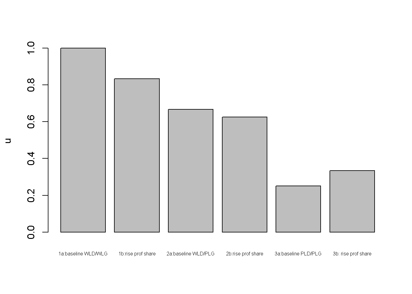
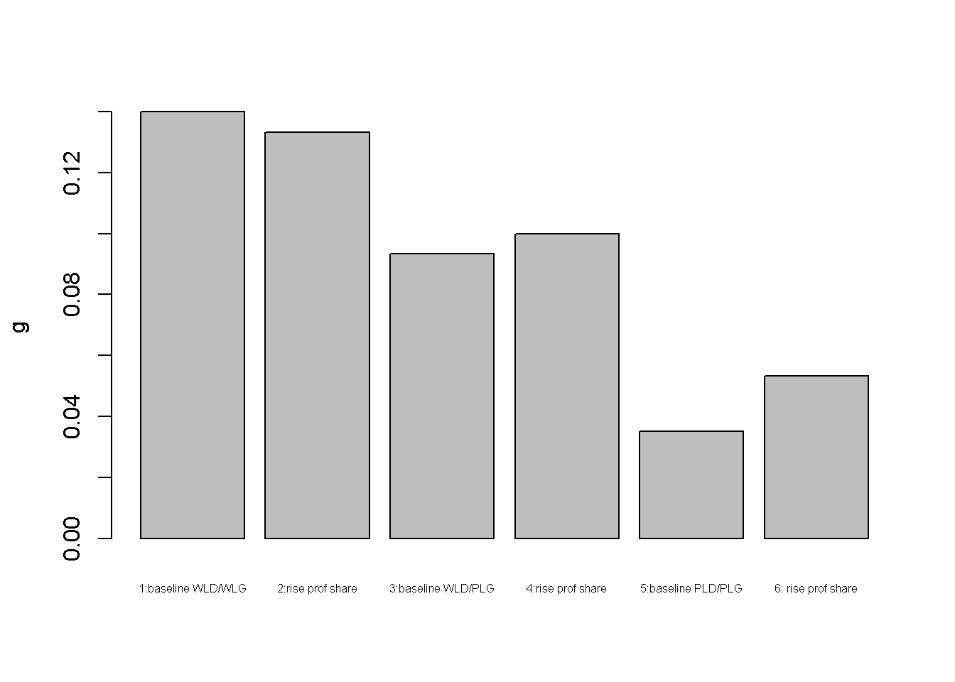
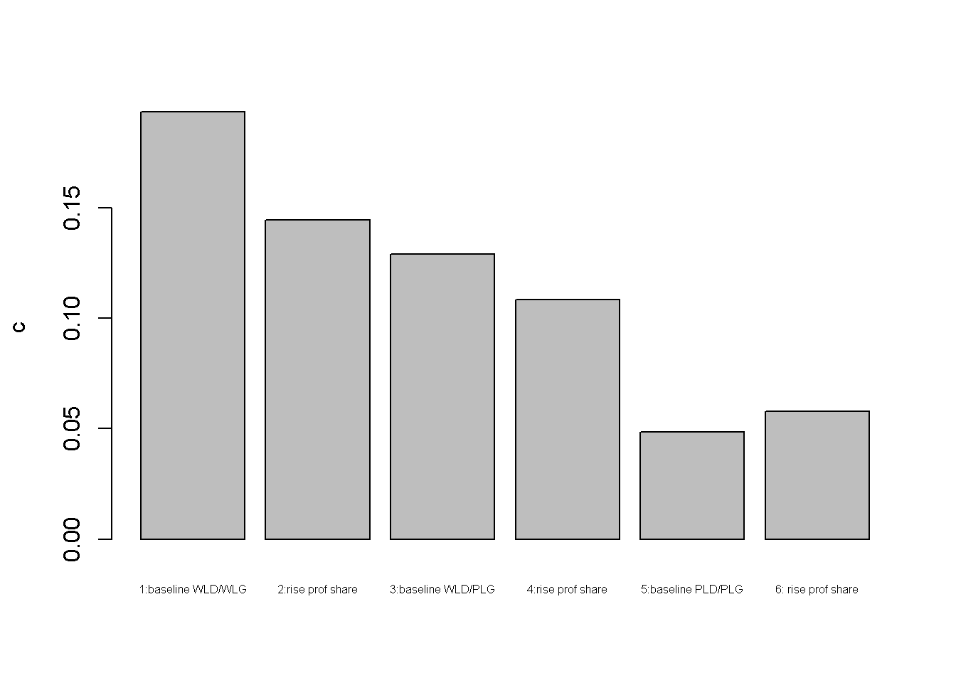
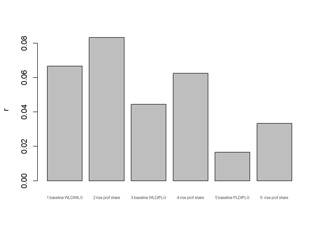
Figures Figure 8.1 - Figure 8.4 depict the response of the model’s key endogenous variables to changes in the profit share. In the first case of a wage-led demand and growth regime (WLD/WLG), investment is equally sensitive to a change in the rate of capacity utilisation (\(g_1\)) and a change in the profit share (\(g_2\)). A rise in the profit share reduces consumption, which reduces the rate of capacity utilisation and the rate of growth. This is despite a positive effect on the profit rate.⁴

barplot(u_star, ylab="u", names.arg=c("1a:baseline WLD/WLG", "1b:rise prof share", "2a:baseline WLD/PLG", "2b:rise prof share", "3a:baseline PLD/PLG", "3b: rise prof share"), cex.names = 0.5)

Figure 8.1: Rate of capacity utilisation

In the second case where the demand regime is wage-led but the growth regime is profit-led (WLD/PLG), investment is slightly less sensitive to a change in the rate of capacity utilisation compared to a change in the profit share. The rise in the profit share reduces consumption and the rate of utilisation, but the ultimate effect on investment is positive because investment reacts more strongly to the rise in the profit share than to the fall in demand.

barplot(g_star, ylab="g", names.arg=c("1:baseline WLD/WLG", "2:rise prof share", "3:baseline WLD/PLG",
                                      "4:rise prof share", 
                                      "5:baseline PLD/PLG", "6: rise prof share"), cex.names = 0.5)

Finally, in the third case where the demand regime and the growth regime are profit-led, investment is again equally sensitive to a change in the rate of capacity utilisation and to a change in the profit share, but now animal spirits are negative. A rise in the profit share now has strong positive effects on investment, which raises the rate of capacity utilisation and consumption.

barplot(c_star, ylab="c", names.arg=c("1:baseline WLD/WLG", "2:rise prof share", "3:baseline WLD/PLG",
                                      "4:rise prof share", 
                                      "5:baseline PLD/PLG", "6: rise prof share"), cex.names = 0.5)

barplot(r_star, ylab="r", names.arg=c("1:baseline WLD/WLG", "2:rise prof share", "3:baseline WLD/PLG",
                                     "4:rise prof share", 
                                     "5:baseline PLD/PLG", "6: rise prof share"), cex.names = 0.5)

Python code

# Plot results (here only for rate of capacity utilisation) 
import matplotlib.pyplot as plt    

# Scenario labels
scenario_names = ["1a: baseline WLD/WLG", "1b: rise prof share", "2a: baseline WLD/PLG", "2b: rise prof share", "3a: baseline PLD/PLG", "3b: rise prof share"]

# Bar plot for u_star
plt.bar(scenario_names, u_star)
plt.ylabel('u')
plt.xticks(scenario_names, rotation=45, fontsize=6)
plt.show()

Directed graph

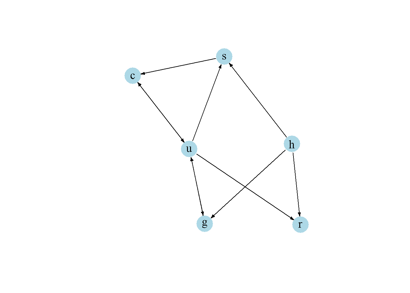
Another perspective on the model’s properties is provided by its directed graph. A directed graph consists of a set of nodes that represent the variables of the model. Nodes are connected by directed edges. An edge directed from a node \(x_1\) to node \(x_2\) indicates a causal impact of \(x_1\) on \(x_2\).

## Create directed graph 
# Construct auxiliary Jacobian matrix for 6 variables: 
# r, h, u, s, c, g

M_mat=matrix(c(0,1,1,0,0,0,
               0,0,0,0,0,0,
               0,0,0,0,1,1,
               0,1,1,0,0,0,
               0,0,1,1,0,0,
               0,1,1,0,0,0), 6, 6, byrow=TRUE)

# Create adjacency matrix from transpose of auxiliary Jacobian 
A_mat=t(M_mat)

# Create and plot directed graph from adjacency matrix
library(igraph)
dg= graph_from_adjacency_matrix(A_mat, mode="directed", weighted= NULL)

# Define node labels
V(dg)$name=c("r", "h", "u", "s", "c", "g")

# Plot directed graph
plot(dg, main="", vertex.size=20, vertex.color="lightblue", 
     vertex.label.color="black", edge.arrow.size=0.3, edge.width=1.1, edge.size=1.2,
     edge.arrow.width=1.2, edge.color="black", vertex.label.cex=1.2, 
     vertex.frame.color="NA", margin=-0.08)

Figure 8.5: Directed graph of post-Kaleckian growth model

Python code

# Load relevant libraries
import networkx as nx
import matplotlib.pyplot as plt
import numpy as np

# Define the Jacobian matrix
M_mat = np.array([[0,1,1,0,0,0],
                  [0,0,0,0,0,0],
                  [0,0,0,0,1,1],
                  [0,1,1,0,0,0],
                  [0,0,1,1,0,0],
                  [0,1,1,0,0,0],
                 ])

# Create adjacency matrix from transpose of auxiliary Jacobian and add column names
A_mat = M_mat.transpose()

# Create the graph from the adjacency matrix
G = nx.DiGraph(A_mat)

# Define node labels
nodelabs = {0: "r", 1: "h", 2: "u", 3: "s", 4: "c", 5: "g"}

# Plot the directed graph
pos = nx.spring_layout(G, seed=43)  
nx.draw(G, pos, with_labels=True, labels=nodelabs, node_size=300, node_color='lightblue', 
        font_size=10)
edge_labels = {(u, v): '' for u, v in G.edges}
nx.draw_networkx_edge_labels(G, pos, edge_labels=edge_labels, font_color='black')
plt.axis('off')
plt.show()

In Figure Figure 8.5, it can be seen that the profit share (\(h\)) is the key exogenous variable of the model.⁵ Consumption (\(c\)), saving (\(s\)), investment (\(g\)), and the rate of utilisation (\(u\)) form a closed loop (or cycle) within the system. The profit share affects both saving and investment, which in turn affect consumption and the rate of capacity utilisation. The profit rate is a residual variable (also called a `sink’) in this model.

Analytical discussion

To find the equilibrium solutions, substitute Equation 8.2 - Equation 8.4 into Equation 8.5 and solve for \(u\): \[\begin{align} u^* = \frac{g_0+g_2h}{[s_W + (s_\Pi - s_W)h]v^{-1}-g_1}. \end{align}\]

The equilibrium solution for \(u\) can then be substituted into Equation 8.4 to find: \[\begin{align} g^* = \frac{(g_0+g_2h)[s_W + (s_\Pi - s_W)h]v^{-1}}{[s_W + (s_\Pi - s_W)h]v^{-1}-g_1}. \end{align}\]

The Keynesian stability condition requires \([s_W + (s_\Pi - s_W)h]v^{-1}-g_1>0\), i.e. saving need to react more strongly to income than investment.

The equilibrium solution for \(r\) can be found by substituting \(u^*\) into Equation 8.1: \[\begin{align} r^* = \frac{h(g_0+g_2h)}{[s_W + (s_\Pi - s_W)h]-vg_1}. \end{align}\]

To assess whether the demand regime is wage- or profit-led, take the derivative of \(u^*\) with respect to \(h\): \[\begin{align} \frac{\partial u^*}{\partial h} = \frac{\frac{s_W}{v}(g_0+g_2 )-(g_0\frac{s_\Pi}{v} + g_1g_2)}{[[s_W + (s_\Pi - s_W)h]v^{-1}-g_1]^2}. \end{align}\]

It can be seen that, e.g., a higher propensity to save out of wages or negative animal spirits make the regime more likely to be profit-led.

By the same token, the sign of the derivative of \(g^*\) with respect to \(h\) determines whether the growth regime is wage- or profit-led: \[\begin{align} \frac{\partial g^*}{\partial h} = g_1\frac{\partial u^*}{\partial h}+g_2. \end{align}\]

It can be seen that, e.g., a higher sensitivity of investment with respect to the profit share makes the regime more likely to be profit-led.

Finally, the effect on the profit rate will depend on the sign of the derivative: \[\begin{align} \frac{\partial r^*}{\partial h} = \frac{u^*}{v} + \frac{h}{v}\frac{\partial u^*}{\partial h}, \end{align}\]

which is likely to be positive but can become negative if the demand regime is strongly wage-led.

Calculate analytical solutions numerically

# Utilisation rate
for (i in 1:S){
print((g0[i]+g2*h[i])/((sw+(sp-sw)*h[i])/v-g1[i]))
}

[1] 1
[1] 0.8333333
[1] 0.6666667
[1] 0.625
[1] 0.25
[1] 0.3333333

# Growth rate
for (i in 1:S){
  print(((g0[i]+g2*h[i])*(sw+(sp-sw)*h[i])/v)/((sw+(sp-sw)*h[i])/v-g1[i]))
}

[1] 0.14
[1] 0.1333333
[1] 0.09333333
[1] 0.1
[1] 0.035
[1] 0.05333333

# Profit rate
for (i in 1:S){
  print((g0[i]+g2*h[i])*(h[i]/v)/((sw+(sp-sw)*h[i])/v-g1[i]))
}

[1] 0.06666667
[1] 0.08333333
[1] 0.04444444
[1] 0.0625
[1] 0.01666667
[1] 0.03333333

Python code

# Utilisation rate
for i in range(S):
    print((g0[i]+g2*h[i])/((sw+(sp-sw)*h[i])/v-g1[i]))

# Growth rate
for i in range(S):
    print(((g0[i]+g2*h[i])*(sw+(sp-sw)*h[i])/v)/((sw+(sp-sw)*h[i])/v-g1[i]))
    
# Profit rate
for i in range(S):
    print((g0[i]+g2*h[i])*(h[i]/v)/((sw+(sp-sw)*h[i])/v-g1[i]))

References

Bhaduri, Amit, and Stephen Marglin. 1990. “Unemployment and the Real Wage: The Economic Basis for Contesting Political Ideologies.” Cambridge Journal of Economics 14 (4): 375–93.

Hein, Eckhard. 2014. Distribution and Growth After Keynes: A Post-Keynesian Guide. Cheltenham: Edward Elgar.

Lavoie, Marc. 2014. Post-Keynesian Economics: New Foundations. Cheltenham; Northampton, MA: Edward Elgar.

See Hein (2014), chap. 7 and Lavoie (2014), chap. 6 for detailed treatments.↩︎
All variables are normalised by the capital stock and thus rendered stationary.↩︎
Bhaduri and Marglin (1990) further discuss the effects on the profit rate.↩︎
If the negative effect on the rate of capacity utilisation was stronger, the profit rate could fall as well. See the analytical discussion for a formal derivation of the condition under which this may happen.↩︎
Other important exogenous variables or parameters that may shift but are not depicted here are animal spirits (\(g_0\)) or the saving propensities (\(s_W, s_\Pi\)). See Hein (2014), chap. 7.2.2, for a detailed discussion of their effects.↩︎