In the 1950s and 1960s in Cambridge UK, Nicholas Kaldor and Joan Robinson developed a theory of growth that aimed to apply John Maynard Keynes’ principle of effective demand to the long run.1 The main Keynesian assumption retained by Kaldor and Robinson was that investment and saving are independent, and that a change in investment may lead to an adjustment in saving. However, unlike Keynes, Kaldor and Robinson assumed a fixed level of capacity utilisation, which they considered a key feature of a long-run equilibrium. As a result, goods market clearing cannot be established via output adjustment. Instead, Kaldor and Robinson assumed price adjustment, which would translate into a change in income distribution. Changes in the distribution of income then affect consumption (and saving), as workers tend to have a higher marginal propensity to consume than capital owners. For example, an increase in investment demand due to improved animal spirits would then lead to excess demand, which raises the price level. For a given level of nominal wages, the rise in the price level lowers real wages, leading to a redistribution of income towards profits. The resulting rise in the profit share increases aggregate saving, thereby leading to an adjustment of saving to investment. Taken together, the Kaldor-Robinson approach highlights the relevance of supply constraints in the long run that can lead to inflationary outcomes of demand shocks.
We consider a simple version of the model proposed in Hein (2014), chap. 4.4. This is a model of long-run steady state growth. In the steady state, all endogenous variables grow at the same rate.2 Changes in parameters or exogenous variables lead to an instantaneous adjustment of the model’s variables, so that the model can be analysed like a static one. The key question addressed by this model is a how changes in aggregate demand affects income distribution and the rate of growth.
The Model
\[
r=h \frac{u_n}{v}
\tag{7.1}\]
\[
s=s_\Pi r, \quad s_\Pi \in (0,1)
\tag{7.2}\]
\[
c= \frac{u_n}{v}-s
\tag{7.3}\]
\[
g=g_0+g_1r, \quad g_1 > 0
\tag{7.4}\]
\[
h=\frac{vg_0}{u_n(s_\Pi-g_1)}
\tag{7.5}\]
where \(r\), \(s\), \(c\), \(g\), and \(h\) are the profit rate, the saving rate, the consumption rate, the investment rate, and the profit share, respectively.
Equation 7.1 decomposes the profit rate into the product of the profit share \(h\) (total profits over total output), the normal rate of capacity utilisation (\(u_n\)), and the inverse of \(v\) (the capital-potential output ratio). Let \(Y\) be output, \(K\) be the capital stock, and \(Y^P\) be potential output, then the decomposition can also be written as \(r=\frac{\Pi}{K}=\frac{\Pi}{Y}\frac{Y}{Y^P}\frac{Y^P}{K}\). The normal rate of capacity utilisation and the capital-potential output ratio are taken to be exogenous in this model. Note also that the wage share is given by \(1-h\). By Equation 7.2, the economy-wide saving rate is given by saving out of profits (\(s_\Pi r\)). It is assumed that workers don’t save, i.e. have a higher marginal propensity to consume than capital owners. Equation 7.3 simply states that consumption is income not saved. According to Equation 7.3, investment is determined by an autonomous component \(g_0\) that may capture Keynesian ‘animal spirits’ and by the profit rate. The profit rate may stimulate investment if firms use adaptive expectations and predict higher future profits in response to an increase in the current profit rate. Finally, Equation 7.5 is the goods market equilibrium condition \(g=s\) solved for the profit share, reflecting the fact that prices are assumed to clear the goods market which translates into an adjustment of the profit share.
Simulation
Parameterisation
Table 1 reports the parameterisation used in the simulation. We will consider three different parameterisations. Besides a baseline scenario (labelled as scenario 1), we will consider an increase in animal spirits (\(g_0\)) and an increase in the propensity to save out of profits (\(s_\Pi\)).
Table 1: Parameterisation
Scenario
\(v\)
\(s_\Pi\)
\(g_0\)
\(g_1\)
\(u_n\)
1: baseline
3
0.6
0.02
0.3
0.9
2: rise in animal spirits (\(g_0\))
3
0.6
0.04
0.3
0.9
3: rise in saving propensity (\(s_\Pi\))
3
0.9
0.02
0.3
0.9
Simulation code
#Clear the environmentrm(list=ls(all=TRUE))# Set number of scenarios (including baselines)S=3#Create vector in which equilibrium solutions from different parameterisations will be storedh_star=vector(length=S)# profit shareg_star=vector(length=S)# growth rate of capital stocks_star=vector(length=S)# saving ratec_star=vector(length=S)# consumption rater_star=vector(length=S)# profit rate# Set constant parameter valuesv=3# capital-to-potential output ratiog1=0.3# sensitivity of investment with respect to profit rate un=0.9# normal rate of capacity utilisation# Set exogenous variables whose parameterisation changes across regimes g0=vector(length=S)# animal spiritssp=vector(length=S)# propensity to save out of profits### Construct different scenarios # scenario 1: baseline g0[]=0.02sp[]=0.6#scenario 2: increase in animal spiritsg0[2]=0.04# scenario 3: increase in propensity to save out of profitssp[3]=0.9#Check stability condition for all scenariosfor(iin1:S){print(sp[i]>g1)}
[1] TRUE
[1] TRUE
[1] TRUE
# Initialise endogenous variables at some arbitrary positive value g=r=s=c=h=1#Solve this system numerically through 1000 iterations based on the initialisationfor(iin1:S){for(iterationsin1:1000){#(1) Profit rater=(h*un)/v#(2) Savings=sp[i]*r#(3) Consumptionc=un/v-s#(4) Investmentg=g0[i]+g1*r#(5) Goods market equilibrium profit shareh=(v/un)*(g0[i]/(sp[i]-g1))}#Save results for different parameterisations in vectorh_star[i]=hg_star[i]=gr_star[i]=rs_star[i]=sc_star[i]=c}
Python code
import numpy as np# Clear the environment (not necessary in Python)# Set number of scenarios (including baselines)S =3# Create arrays to store equilibrium solutions for different parameterizationsh_star = np.empty(S) # profit shareg_star = np.empty(S) # growth rate of capital stocks_star = np.empty(S) # saving ratec_star = np.empty(S) # consumption rater_star = np.empty(S) # profit rate# Set constant parameter valuesv =3# capital-to-potential output ratiog1 =0.3# sensitivity of investment with respect to profit rate un =0.9# normal rate of capacity utilization# Set exogenous variables whose parameterization changes across regimesg0 = np.empty(S) # animal spiritssp = np.empty(S) # propensity to save out of profits# Construct different scenarios# Scenario 1: baselineg0[:] =0.02sp[:] =0.6# Scenario 2: increase in animal spiritsg0[1] =0.04# Scenario 3: increase in propensity to save out of profitssp[2] =0.9# Check stability condition for all scenariosfor i inrange(S):print(sp[i] > g1)# Initialize endogenous variables at some arbitrary positive valueg = r = s = c = h =1# Solve this system numerically through 1000 iterations based on the initializationfor i inrange(S):for iterations inrange(1000):# (1) Profit rate r = (h * un) / v# (2) Saving s = sp[i] * r# (3) Consumption c = un / v - s# (4) Investment g = g0[i] + g1 * r# (5) Goods market equilibrium profit share h = (v / un) * (g0[i] / (sp[i] - g1))# Save results for different parameterizations in arrays h_star[i] = h g_star[i] = g r_star[i] = r s_star[i] = s c_star[i] = c
Plots
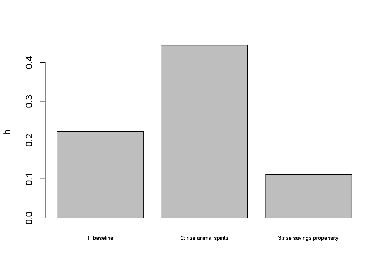
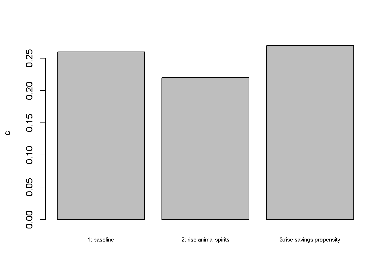
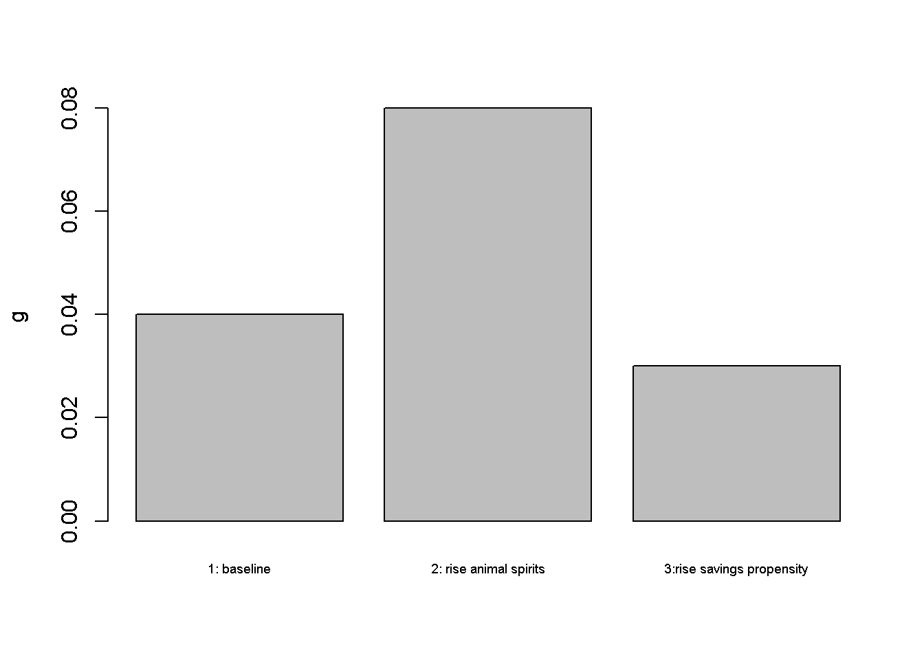
Figures Figure 7.1 - Figure 7.3 depict the response of the model’s key endogenous variables to changes in aggregate demand. A rise in animal spirits (scenario 2) raises the profit share. This reduces consumption. However, the effect on capital accumulation and thus growth is positive. In that sense, long-run growth is demand-driven, despite the fixed rate of capacity utilisation.
In the second scenario, the saving propensity of capital owners increases. This constitutes a reduction in aggregate demand, leading to a fall in the profit share, and a fall in the growth rate. Since \(g=s\), the effect reflects the Keynesian ‘paradox of saving’: a rise in the saving propensity leads to a fall in the aggregate saving rate.
# Plot results (here only for profit share) import matplotlib.pyplot as plt# Scenario labelsscenario_names = ["1: baseline", "2: rise animal spirits", "3: rise savings propensity"]# Bar plot for h_starplt.bar(scenario_names, h_star)plt.ylabel('h')plt.xticks(scenario_names, rotation=45, fontsize=6)plt.show()
Directed graph
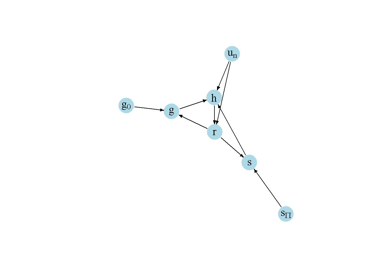
Another perspective on the model’s properties is provided by its directed graph. A directed graph consists of a set of nodes that represent the variables of the model. Nodes are connected by directed edges. An edge directed from a node \(x_1\) to node \(x_2\) indicates a causal impact of \(x_1\) on \(x_2\).
Figure 7.4: Directed graph of Kaldor-Robinson growth model
Python code
# Load relevant librariesimport networkx as nximport matplotlib.pyplot as pltimport numpy as np# Define the Jacobian matrixM_mat = np.array([[0, 1, 0, 0, 0, 0, 1], [0, 0, 1, 1, 0, 0, 1], [1, 0, 0, 0, 0, 1, 0], [1, 0, 0, 0, 1, 0, 0], [0, 0, 0, 0, 0, 0, 0], [0, 0, 0, 0, 0, 0, 0], [0, 0, 0, 0, 0, 0, 0]])# Create adjacency matrix from transpose of auxiliary Jacobian and add column namesA_mat = M_mat.transpose()# Create the graph from the adjacency matrixG = nx.DiGraph(A_mat)# Define node labelsnodelabs = {0: "r", 1: "h", 2: "s", 3: "g", 4: r"$g_0$", 5: r"$s_p$", 6: r"$u_n$"}# Plot the directed graphpos = nx.spring_layout(G, seed=43) nx.draw(G, pos, with_labels=True, labels=nodelabs, node_size=300, node_color='lightblue', font_size=10)edge_labels = {(u, v): ''for u, v in G.edges}nx.draw_networkx_edge_labels(G, pos, edge_labels=edge_labels, font_color='black')plt.axis('off')plt.show()
In Figure Figure 7.4, it can be seen that animal spirits (\(g_0\)), the propensity to save out of profits (\(s_\Pi\)), and the normal rate of capacity utilisation (\(u_n\)) are the key exogenous variable of the model. Saving (\(s\)), investment (\(g\)), the rate of profit (\(r\)), and the profit share (\(h\)) are endogenous and form a closed loop (or cycle) within the system.